Explore, play, analyse your corpus with TXM

A short introduction of TXM by José Calvo Tello and Silvia Gutiérrez

On Feburary 6-7, 2014, the Department for Literary Computing, Würzburg University, organized a DARIAH-DE Workshop called „Introduction to the TXM Content Analysis Platform„. The workshop leader was Serge Heiden (ENS-Lyon) who is in charge of the conceptualizing and implementing TXM at the ICAR Laboratory in France.

The workshop included a brief explanation of TXM’s background, but it concentrated on a very practical approach. We learned about the “Corpora options” (that is what you can know about your corpus: POS descriptions, text navigation), but also what you can do with it: find Key Words In Context (KWIC), retrieve Parts of Speech, and moreover how you can analyse these results querying for the Most Frequent Words or the cooccurrences.

In the evening of day one, we got an overview of the state of art of the use of „Natural Language Processing for Historical Texts“ in a keynote by Michael Piotrowski (IEG Mainz). First of all, he started by defining Historical Texts as all those texts that will bring major problems to NLP. In order to clarify these definitions, Dr. Piotrowski listed some of the greatest difficulties:

• Medium and integrity: we have to remember that in order to analyse an old script that was written in clay tablets or marble, it is compulsory to first find a way to transfer this information into a digital format (not an easy task); plus: some texts are defective or unclear, and transcriptions may introduce new errors
• Language, writing system and spelling: many of the historical texts were written in extinct languages or variants different from today’s variants; as for the writing system, the many abbreviation forms and the variety of typefaces are more or less problematic; finally, we should not forget the little problem of non-standardized spelling!
• State of art: Historical languages are less-resourced-languages, there are few texts available, and NLP for historical languages is carried out in specific projects; that is, there are no common standards and everyone has to start from zero.

Not to discourage his public, he then offered an overview of what can be done: Part-of-speech tagging. Creating a tagger for a historical language can be done with the the following methods:

1. From scratch: manually annotating your text
2. Using a modern tagger and manually correcting all errors
3. Modernizing spelling
4. Bootstraping POS tagger (with many versions of the same text, like the Bible)

Now let’s get back to the TXM workshop. In this post, you will find a brief practical introduction to this tool. We will provide you with a rough idea of what is this software about and what you can do with it. If you would like to learn more, do check the links we have shared towards the end of this post. By the way, all words marked with a little * are explained at the end, in the “Vocabulary” section.

What is TXM?

This software is at the juncture of linguistics and scholarly editing and it’s made to help scholars analyse the content of any kind of digital text (Unicode encoded raw texts or XML/TEI tagged texts).

To get to know more about the TXM background, don’t miss Serge Heiden’s Workshop slides:

Where can I work with it?

You may work on the desktop (download page) or online version of the tool. Both platforms have advantages and disadvantages. The online version allows you to start the work without downloading or installing anything, and share your corpora with other colleagues. With the desktop version, you can easily lemmatize and analyse the Parts of Speech (POS*) of your own texts.

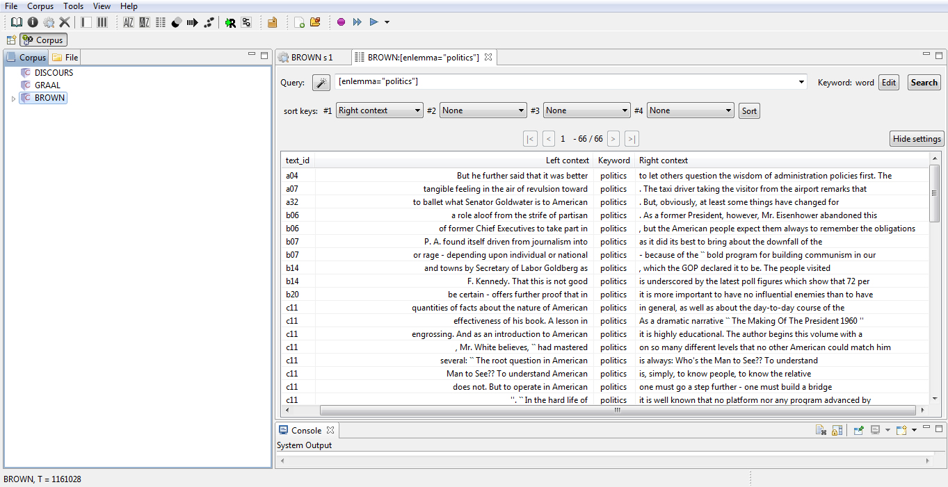
So that you can get a better idea of the way it works, we’ll guide you with some practical examples. Say you want to search for the lemma politics on the „Brown Corpus*. First you have to open the Index option:

Then you use the query box to type in the query, using the following structure from the CQL* query language: [enlemma=“politics”]. In the desktop version, the results will look as follows (the web version is very similar):

What can I do with TXM?

Explore your corpus

Corpora options

On the first column of both interfaces there’s a list of the corpora you can work with (in this case DISCOURS, GRAAL, BROWN). When you click with the right button of your mouse on one of your corpora, you will see a list of icons:

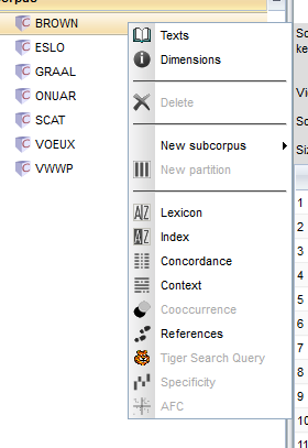
These are the main tools of TXM and you will use one of these to analyse your corpus in different ways.

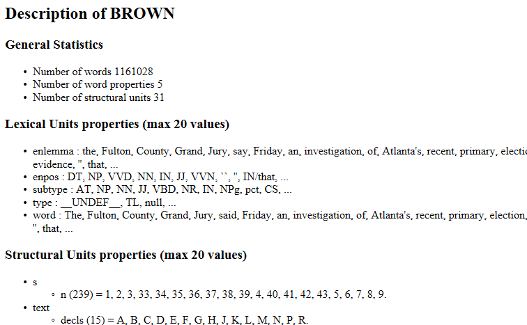
Corpus description (Dimensions)

Before you start with the fun, you should click the “Dimensions” option and have a look at some general information about the corpus (number of words, properties, and structural units, as well as the lexical and structural units properties). This information is richer in the desktop version:

Text navigation

A very practical TXM feature is the text display. If you wish to open a list of the corpus’ elements, you just have to click on the book icon (called “Texts” in the online version and “Open edition” in the other). A list like the following will be shown:

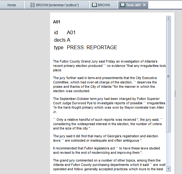
Moreover, if you click on the book icon in the “edition” column, TXM will open a readable version of our text:

Play with your corpus

Key Words In Context (KWIC)

A very typical visualization of a corpus is the so called KWIC view, which you have already seen displayed in the politics lemma example.

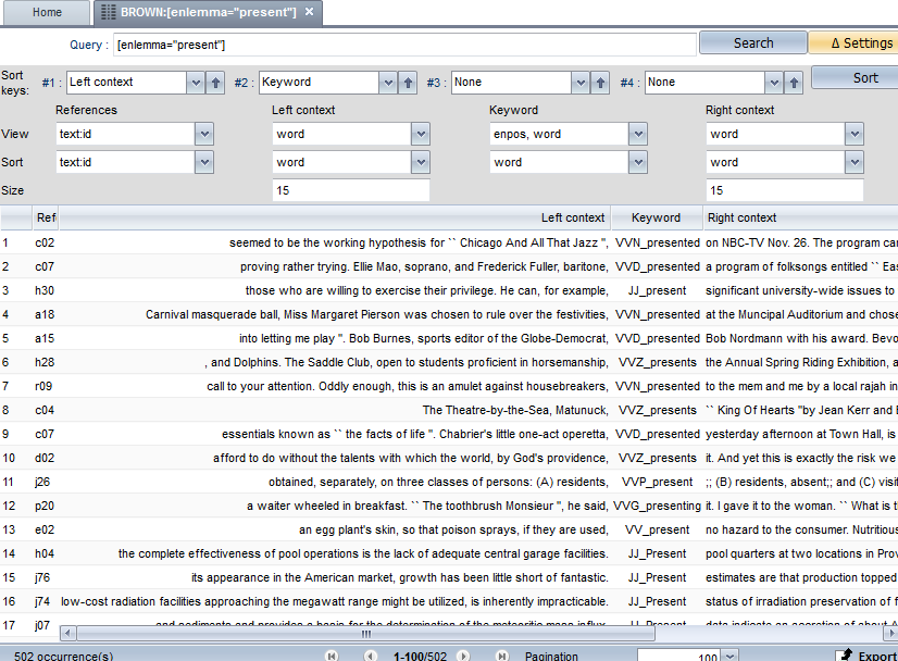
With TXM you can sort the results using different criteria organizing them according to the right or left context of your word, the word form, etc; besides, you can choose which elements you want to visualize. Say you’re searching for collocations of present as an adjective and NOT the data related to the noun nor the verb form (to present). First of all you need to go to the INDEX.

Once you open this, you can set the options in the “Keyword” column and visualize the grammatical category along with the word form. Then you type „JJ_present“, where „JJ“ means „adjective“ and „present“ is the verb form, so that only those instances of the graphical form present are selected which are adjectives. It is also possible to order this data by different criteria.

As you can see in the next screenshot, you are looking for the lemma present. Therefore, you should set the first “Sort keys” menu to “Left context”, and the second one to “Keyword”; what you’re saying to the software is that you want all the examples sorted by the Left context as a first criteria and the Keyword as a second. In the “Keyword” > “View” menu we have set “enpos, word”. With that we are ordering TXM to show us not just the word form, but also the POS. That is why we see the keywords as “VVN_present” (that means, present as a verb) or JJ_present (present as an adjective):

Parts of Speech

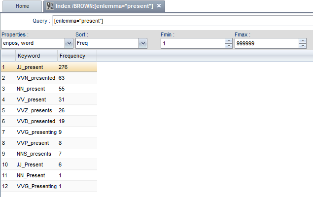
Another way to display specific words according to their POS can be run by using the Index tool (A|Z icon), from a lexicologist point of view one the most interesting options of TXM. If you search again for the lemma present and in the properties box, you chose to see not only the word form but the POS as well, TXM will tell you the frequency, word form and POS of each different word form found in the corpus:

If you only want the word forms of the verb to present, you can add the POS information to the query: [enlemma=“present” & enpos=“VV.*”]

These index can able to create lists of n-grams. Let’s search for the most frequent words that appear after the lemma present:

Quantative analysis

Most Frequent Words

To query something you have to have a specific question and know some basic information, for instance: in which language is the corpus? A way to have a general idea about the texts is the Lexicon option, the icon with AZ both on white background. When you click on it, you will see a list of the most frequent word forms:

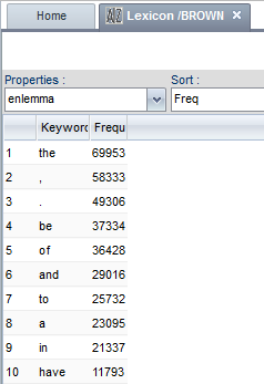
You can change the settings of the query and ask to count not the word forms but the lemmas. In that case the verb to be climbs up some positions, now that is, are, were, been etc. count as one single unity:

Coocurrences

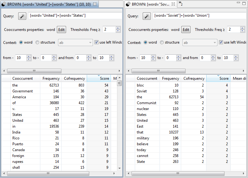
Another quantitative analysis concerns the coocurrences, that is, the words (or other unities) that frequently appear close to a specific word (or to other unities). Unlike n-grams, coocurrences do not have to appear exactly after or before the unity, they just have to be somewhere close to it.

The Brown corpus was compiled in the 1960s in the United States, the main years of the Cold War. So let’s see the vocabulary related to the words United States and which one to Soviet Union:

Progression

Another statistical option that exists on the Desktop version is the Progression (icon with an arrow). This option helps visualize how many times a unity appears in a corpus or a text. This might be interesting to see the progress of a word between two dates or see the development of a word in the different parts of a text.

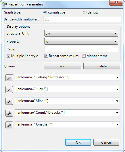
For the next example, the text of Bram Stocker’s novel Dracula was imported (the version used is from the University of Adelaide). With the information of the chapters kept in XML elements, you can look for the name of the main characters and see how many times and where they appear. The next screen-shot shows the complete query:

To understand the next graphic, you have to keep in mind that if the lines ascends, that means the name has been mentioned; if the line keeps going horizontally, it means the name didn’t appear any more.

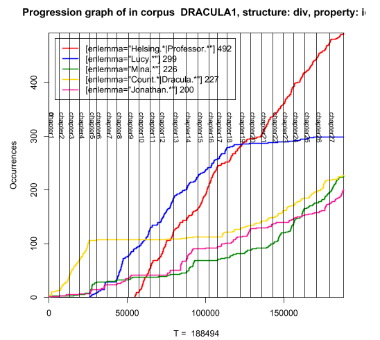
As you can see, the Count Dracula (yellow) is the most mentioned name in the first four chapters, but it almost disappears towards the 17th chapter. In this gap, Lucy (blue) becomes the main character and, from the 9th chapter, the Professor van Helsing (red) takes the “leading” role. It is also remarkable that this last character is not only the most frequent, but the most stable.

Sub-corpora and partitions

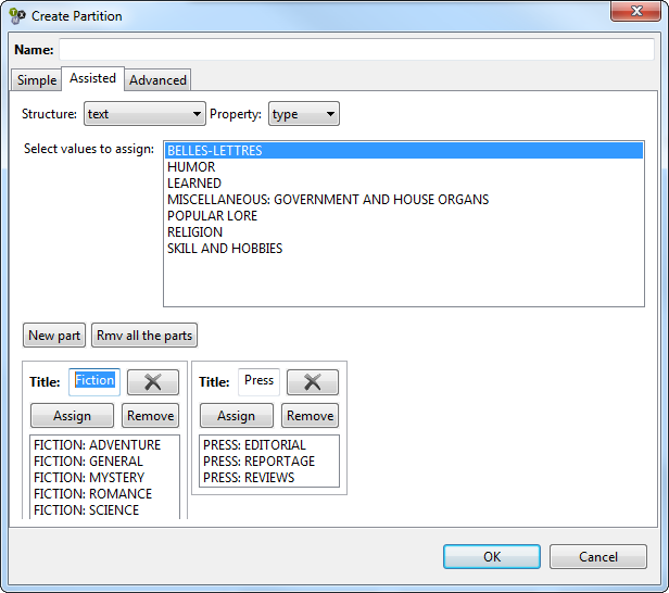
You can divide your corpus into two options: sub-corpora and partitions. With a sub-corpus you can choose some texts from a corpus and work with them. With the partition, you can split the corpus into more than one part and easily compare the results of the different parts. On the next screenshot, you have the menu where a Partition called “Fiction and Press partition” is being created, using the XML “text” and the property “type” to choose which kind of text is wanted. This partition will have two parts: one called “Fiction” and the other one called “Press” and each of it will contain the respective type of texts.

Useful links

“A gentle introduction to TXM key concepts in 90 minutes” by Serge Heiden: http://sourceforge.net/projects/txm/files/documentation/IQLA-GIAT%202013%20TXM-workshop.pdf/download

Tutorial video introducing TXM 0.4.6 (WARNING: the software, specially it’s surface, is now very different): http://textometrie.ens-lyon.fr/IMG/html/intro-discours.htm

TXM background http://fr.slideshare.net/slheiden/txm-background

TXM import process http://fr.slideshare.net/slheiden/txm-import-process

Vocabulary

Brown Corpus

The Brown corpus consists of 500 English-language texts, with roughly one million words, compiled from works published in the United States in 1961. You can learn more about it here.

CQL

TXM uses an underlying Contextual Query Language, which is a formal system for representing queries to information retrieval systems such as web indexes, bibliographic catalogues and museum collection information. It is based on CQP (Corpus Query Processor) developed in Stuttgart. More information under http://cwb.sourceforge.net/files/CQP_Tutorial/

POS

Here is a useful alphabetical list of part-of-speech tags used in the Penn Treebank Project (tag and description): https://www.ling.upenn.edu/courses/Fall_2003/ling001/penn_treebank_pos.html